Plot method for bayesianVARs_bvar

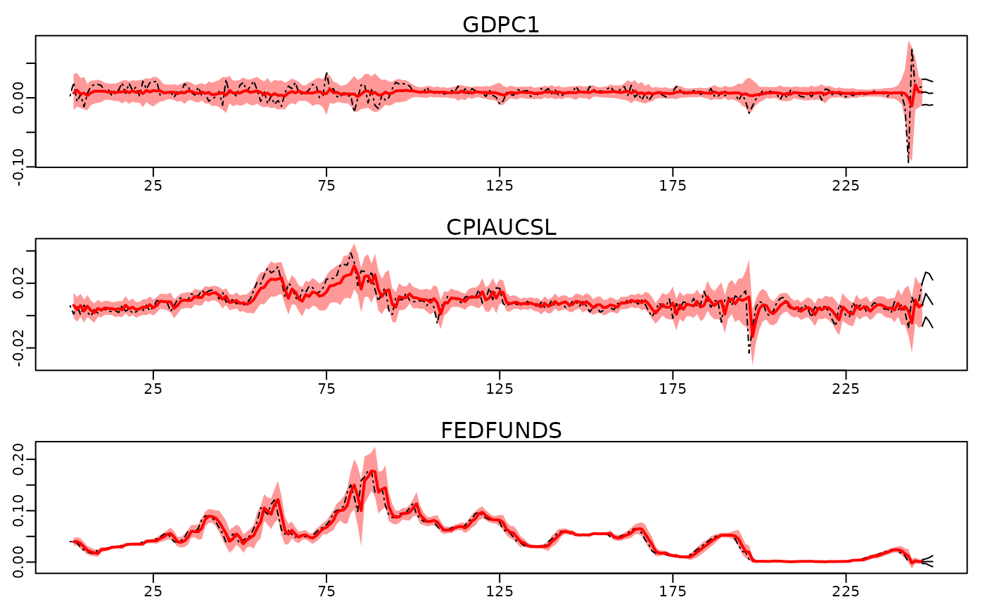
Visualization of in-sample fit. Can also be used to display prediction intervals of future values.

Usage

# S3 method for class 'bayesianVARs_bvar'
plot(
  x,
  predictions = NULL,
  quantiles = c(0.05, 0.5, 0.95),
  dates = NULL,
  n_col = 1,
  ...
)

Arguments

x

An object of class bayesianVARs_bvar obtained via bvar().

predictions

Optional array of out of sample predictions, e.g. obtained via predict.bayesianVARs_bvar().

quantiles

numeric vector indicating which quantiles to plot.

dates

optional vector of dates for labelling the x-axis. The default values is NULL; in this case, the axis will be labeled with numbers.

n_col

integer indicating the number of columns to use for plotting.

...

Currently ignored!

Value

Returns x invisibly.

See also

Other plotting plot.bayesianVARs_fitted(), plot.bayesianVARs_predict(), pairs.bayesianVARs_predict(), posterior_heatmap().

Examples

# Access a subset of the usmacro_growth dataset
data <- usmacro_growth[,c("GDPC1", "CPIAUCSL", "FEDFUNDS")]

# Estimate a model
mod <- bvar(data, sv_keep = "all", quiet = TRUE)

# Simulate from posterior predictive
predictions <- predict(mod, ahead = 1:3)
#> 'stable=TRUE': Calling 'stable_bvar()' to discard those posterior
#>           draws, that do not fulfill the stable criterion.
#> 
#>  626 stable posterior draws remaining for prediction!

# Visualize
plot(mod, predictions = predictions)