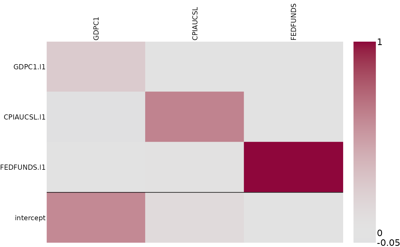
Posterior heatmaps for matrix valued parameters

posterior_heatmap() generates a heatmap for draws of matrix values parameters visualizing point wise summaries, such as mean, median, variance, standard deviation, interquartile range etc. etc.

Usage

posterior_heatmap(
  x,
  FUN,
  ...,
  transpose = FALSE,
  colorbar = TRUE,
  colorbar_width = 0.1,
  gap_width = 0.25,
  xlabels = NULL,
  ylabels = NULL,
  add_numbers = FALSE,
  zlim = NULL,
  colspace = NULL,
  border_color = NA,
  zero_color = NA,
  main = "",
  detect_lags = TRUE,
  cex.axis = 0.75,
  cex.colbar = 1,
  cex.numbers = 1,
  asp = NULL
)

Arguments

x: An array of dimension \(a \times b \times draws\), where \(a \times b\) is the dimension of the parameter to visualize and draws is the number of posterior draws.
FUN: The summary function to be applied to margins c(1,2) of x. E.g. "median", "mean", "IQR", "sd" or "var". apply(x, 1:2, FUN, ...) must return a matrix!
...: optional arguments to FUN.
transpose: logical indicating whether to transpose the matrix or not, i.e. whether to plot an \(a \times b\) or an \(b \times a\) matrix. Default is FALSE.
colorbar: logical indicating whether to display a colorbar or not. Default is TRUE.
colorbar_width: numeric. A value between 0 and 1 indicating the proportion of the width of the plot for the colorbar.
gap_width: numeric. A value between 0 and 1 indicating the width of the gap between the heatmap and the colorbar. The width is computed as gap_width*colorbar_width.
xlabels: ylabels=NULL, the default, indicates that colnames(x) will be displayed. ylabels="" indicates that no ylabels will be displayed.
ylabels: xlabels=NULL, the default, indicates that rownames(x) will be displayed. xlabels="" indicates that no ylabels are displayed.
add_numbers: logical. add_numbers=TRUE, the default indicates that the actual values of summary will be displayed.
zlim: numeric vector of length two indicating the minimum and maximum values for which colors should be plotted. By default this range is determined by the maximum of the absolute values of the selected summary.
colspace: Optional argument indicating the color palette to be used. If not specified, colorspace::diverge_hcl() will be used, or, if FUN returns only positive values colorspace::sequential_hcl(). See below for a more detailed description of the default usage.
border_color: The color of the rectangles borders. If not specified no borders will be displayed.
zero_color: The color of exact zero elements. By default this is not specified and then will depend on colspace.
main: main title for the plot.
detect_lags: logical. If class(x) is "bayesianVARs_coef", then detect_lags=TRUE will separate the sub matrices corresponding to the lags with black lines.
cex.axis: The magnification to be used for y-axis annotation relative to the current setting of cex.
cex.colbar: The magnification to be used for colorbar annotation relative to the current setting of cex.
cex.numbers: The magnification to be used for the actual values (if add_numbers=TRUE) relative to the current setting of cex.
asp: aspect ratio.

Value

Returns x invisibly.

Details

colspace

If not specified either colorspace::diverge_hcl(1001, alpha = alpha, palette = "Blue-Red") or colorspace::sequential_hcl(1001, alpha = alpha, rev = TRUE, palette = "Reds 2") will be used.

Examples

# Access a subset of the usmacro_growth dataset
data <- usmacro_growth[,c("GDPC1", "CPIAUCSL", "FEDFUNDS")]

# Estimate a model
mod <- bvar(100*data, sv_keep = "all", quiet = TRUE)

# Extract posterior draws of VAR coefficients
phi_post <- coef(mod)

# Visualize posterior median of VAR coefficients
posterior_heatmap(phi_post, median, detect_lags = TRUE, border_color = rgb(0, 0, 0, alpha = 0.2))


# Extract posterior draws of variance-covariance matrices (for each point in time)
sigma_post <- vcov(mod)
# Visualize posterior interquartile-range of variance-covariance matrix of the first observation
posterior_heatmap(sigma_post[1,,,], IQR)