This vignette only deals with the computational complexity of the implemented algorithms. It does not cover sampling efficiency in terms of mixing.
bayesianVARs’ bvar() implements state of the art Markov Chain Monte Carlo (MCMC) algorithms for posterior estimation of Bayesian vectorautoregressions (VARs). The computational complexity of those algorithms depends on the configuration of the error variance-covariance matrix which is specified through the function argument prior_sigma. This argument expects a bayesianVARs_prior_sigma object which can be conveniently created using the helper function specify_prior_sigma().
Factor specification
The factor structure on the errors is achieved by setting specify_prior_sigma()’s argument type = "factor". The following code snippet is a minimal working example of estimating a VAR featuring stochastic volatility with a factor structure on the errors.
set.seed(321)
# Simulate data
n <- 50L # number of observations
M <- 3L # number of time series
Y <- matrix(rnorm(n*M), n, M)
colnames(Y) <- paste0("y", 1:M)
# Estimate a VAR with a factor structure on the errors
prior_sigma_f <- specify_prior_sigma(Y, type = "factor")
mod_f1 <- bvar(Y, draws = 50L, burnin = 5L, prior_sigma = prior_sigma_f,
            quiet = TRUE)
For the factor specification bayesianVARs implements the conditional equation per equation algorithm described in Kastner and Huber (2020). Using default settings, this algorithm is of complexity , where is the number of time series and the number of lags.
Factor specifcation in huge dimensions
In the aforementioned paper it is also demonstrated that for VARs in huge dimensions, within the conditional equation per equation algorithm, the algorithm of Bhattacharya, Chakraborty, and Mallick (2016) for sampling from high-dimensional Gaussian distributions can be exploited to further speed up computations. This feature is invoked by setting bvar()’s argument expert_huge = TRUE.
mod_f2 <- bvar(Y, draws = 50L, burnin = 5L, prior_sigma = prior_sigma_f,
               expert_huge = TRUE, quiet = TRUE)
Using this sampler-configuration, the algorithm is of complexity , where is the number of observations. Therefore, it can be expected that setting expert_huge = TRUE only speeds up computations in scenarios where , i.e. the number of VAR coefficients per equations exceeds the number of observations.
Cholesky specification
The Cholesky structure on the errors is achieved by setting specify_prior_sigma()’s argument type = "cholesky". The following code snippet is a minimal working example of estimating a VAR featuring stochastic volatility with a Cholesky structure on the errors.
# Estimate a VAR with a Cholesky structure on the errors
prior_sigma_c <- specify_prior_sigma(Y, type = "cholesky")
mod_c <- bvar(Y, draws = 50L, burnin = 5L, prior_sigma = prior_sigma_c,
            quiet = TRUE)
For the Cholesky specification bayesianVARs implements the correct triangular algorithm described in Carriero et al. (2022). This algorithm is of complexity , i.e. it has the same complexity like the standard conditional equation per equation algorithm for the factor specification, see Factor specification.
Empirical demonstration
The following code chunk runs the posterior sampling algorithm and records computation times for all sampling algorithms considering all combinations of , , , and .
set.seed(123)
ps <- 1:5 # lags
M <- 50L # number time series
n <- 100L # number of observations for estimation
factors <- c(1L,50L) # number of factors
huge <- c(FALSE, TRUE) # expert_huge algorithm
svs <- c(FALSE, TRUE) # stochastic volatility
factor_combinations <- expand.grid(p = ps, M = M, n = n, r = factors,
                                expert_huge = huge, sv = svs, type = "factor",
                                stringsAsFactors = FALSE)
cholesky_combinations <- expand.grid(p = ps, M = M, n = n, r = 0,
                                expert_huge = FALSE, sv = svs, type = "cholesky",
                                stringsAsFactors = FALSE)
all_combinations <- rbind(factor_combinations, cholesky_combinations)
Tobs <- all_combinations$n + all_combinations$p # number of total observations
all_combinations <- cbind(all_combinations, Tobs = Tobs, user_time = as.numeric(NA))
for(i in seq_len(nrow(all_combinations))){
  p <- all_combinations$p[i]
  M <- all_combinations$M[i]
  Tob <- all_combinations$Tobs[i]
  r <- all_combinations$r[i]
  expert_huge <- all_combinations$expert_huge[i]
  type <- all_combinations$type[i]
  sv <- all_combinations$sv[i]

  # simulate data
  Y <- matrix(rnorm(Tob*M), Tob, M)
  colnames(Y) <- paste0("y", 1:M)
  # prior configuration
  prior_sigma <- specify_prior_sigma(data = Y, type = type, factor_factors = r,
                                     factor_heteroskedastic = sv,
                                     cholesky_heteroscedastic = sv,
                                     quiet = TRUE)
  # generate posterior draws
  res <- bvar(Y, lags = p, draws = 10L, burnin = 0L,
                            prior_intercept = FALSE,
                            prior_sigma = prior_sigma,
       expert_huge = expert_huge, quiet = TRUE)
  # store user time
  all_combinations$user_time[i] <- res[["bench"]]["user.self"]
}
The estimates of computation time are based on an Intel®Core™i7-10610U processor using one core in combination with a standard single-threaded R installation.
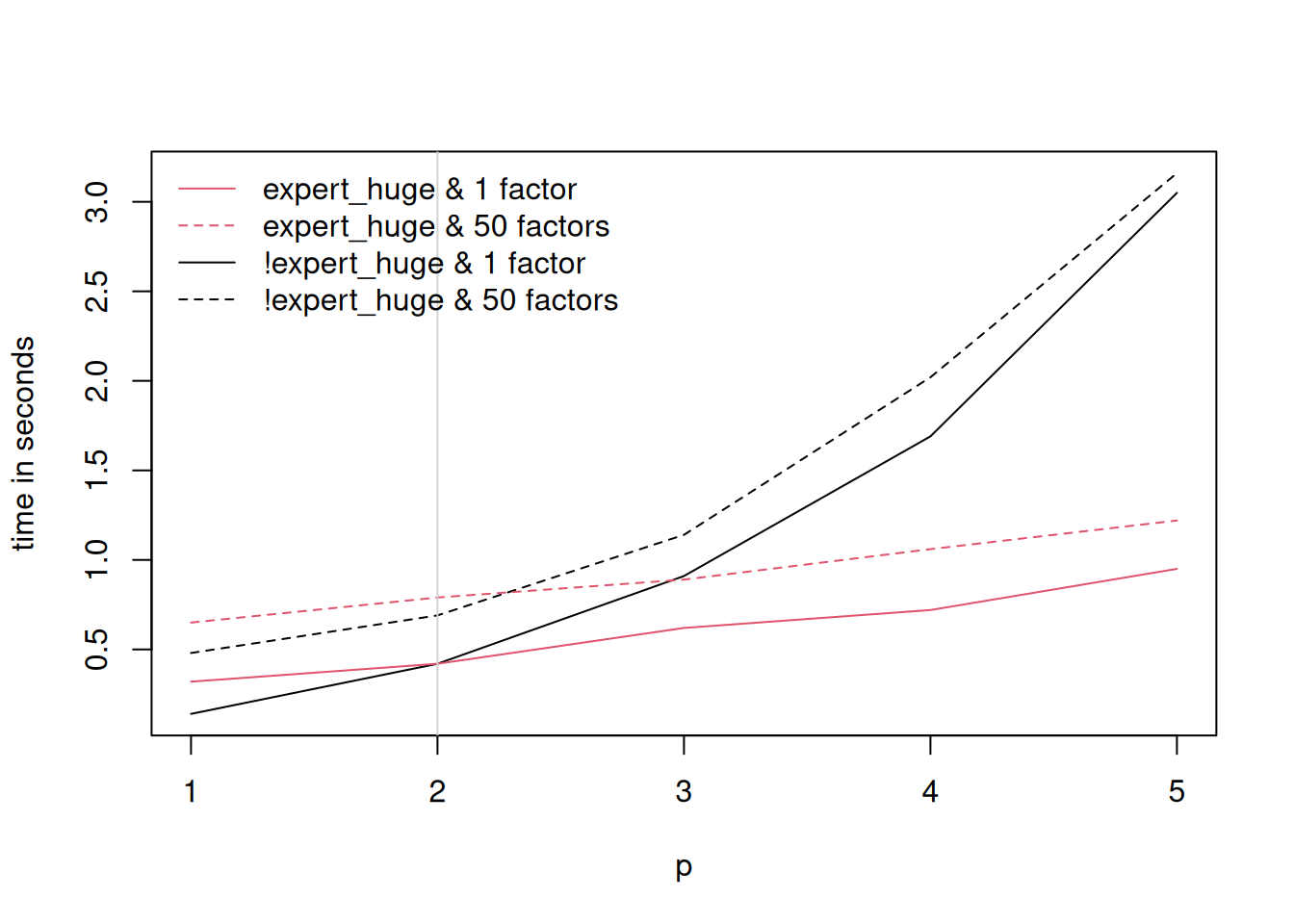
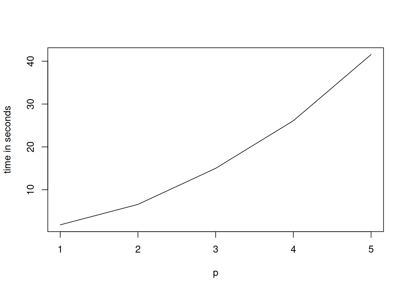
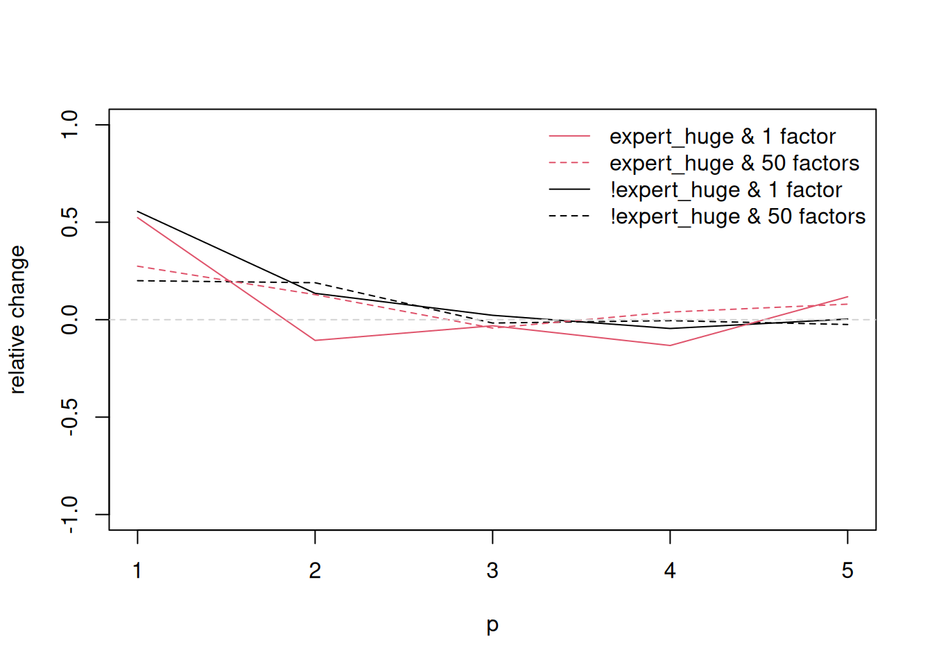
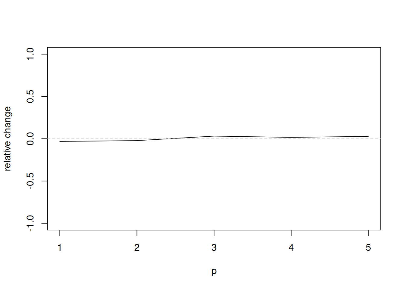
Figure 1, which can be replicated with the following code chunk, depicts the computation time of generating 10 draws from the joint posterior distribution of all parameters and latent variables. Interestingly, the additional cost when moving from a homoscedastic model (constant error variance-covariance matrix) to a heteroscedastic model (time varying error variance-covariance matrix featuring stochastic volatility), or in case of the factor specification when moving from a model with 1 factor to a model with 50 factors, appears to be negligible.
for(type0 in c("factor", "cholesky")){
  tmp <- subset(all_combinations, type == type0 & sv == TRUE)
  plot(0,0, xlim = range(tmp$p), ylim = range(tmp$user_time),
     type="n", xlab = "p", ylab = "time in seconds")
    if(type0=="cholesky"){
      lines(tmp$p,
          tmp$user_time)
    }else{
      for(expert in huge){
        for(rr in factors){
          lines(with(tmp, subset(p, r == rr & expert_huge == expert & type == "factor")),
          with(tmp, subset(user_time, r == rr & expert_huge == expert & type == "factor")),
          col = expert + 1L, lty = if(rr==1L) 1 else 2)
        }
      }
      abline(v = n/M, col = "lightgrey")
      legend("topleft", legend = c("expert_huge & 1 factor", "expert_huge & 50 factors",
                                   "!expert_huge & 1 factor", "!expert_huge & 50 factors"),
             col = c(2L, 2L, 1L, 1L),
             lty = c(1L, 2L, 1L, 2L), bty="n")
    }
}

for(type0 in c("factor", "cholesky")){
  tmp <- subset(all_combinations, type == type0)
  plot(0,0, xlim = range(tmp$p), ylim = c(-1,1),
     type="n", xlab = "p", ylab = "relative change")
  if(type0 == "cholesky"){
    tmp_sv <- subset(tmp, sv == TRUE)
    tmp_nosv <- subset(tmp, sv == FALSE)
    thediff <- tmp_sv$user_time - tmp_nosv$user_time
    normalizer <- tmp_nosv$user_time
    lines(tmp_sv$p, thediff/normalizer)
  }else{
    for(expert in huge){
      for(rr in factors){
        tmp_sv <- subset(tmp, sv == TRUE & r == rr & expert_huge == expert)
        tmp_nosv <- subset(tmp, sv == FALSE & r == rr & expert_huge == expert)
        thediff <- tmp_sv$user_time - tmp_nosv$user_time
        normalizer <- tmp_nosv$user_time
        lines(tmp_sv$p, thediff/normalizer,
          col = expert + 1L, lty = if(rr==1L) 1 else 2)
      }
    }
    legend("topright", legend = c("expert_huge & 1 factor", "expert_huge & 50 factors",
                                 "!expert_huge & 1 factor", "!expert_huge & 50 factors"),
           col = c(2L, 2L, 1L, 1L),
             lty = c(1L, 2L, 1L, 2L), bty = "n")
  }
  abline(h=0, col = "lightgrey", lty=2)

}